About

About This Project

The Equitable Outdoor Access Research Project uses public data to map people and public parks and open spaces. As described in more detail below, we use the Protected Areas Database of the United States to locate public parks and open spaces, and then we use data from the U.S. Census and Meta to map the people who can or cannot access those public lands. 

This project provides a new way to look at access to the outdoors, using detailed data and analysis to show how three specific types of policy interventions can help make access to nature more equitable:

• Expand programming and improve infrastructure to help people reach existing regional parks and open space
• Expand access on existing public lands where access is currently restricted
• Purchase land for new parks and open space 

This project sheds light on the public access objectives of 30x30 conservation goals nationwide. Habitat conservation is another crucial goal of those policies. Our research does not currently incorporate those goals, although future work could combine those objectives. While our research recognizes the importance of building new neighborhood parks in areas where people currently do not have a park within walking distance of their homes, this work focuses on policies to improve access to regional parks and open spaces.

This work analyzes, in unprecedented detail, the “visitorsheds” of parks and open spaces in the United States and then calculates the demographics of the people in those visitorsheds (and outside any visitorshed) to understand where advocates, policymakers, land managers, and others can target investments in programs and infrastructure, opening access to restricted lands, or land acquisitions to make access to the outdoors more equitable. We define a “visitorshed” as the total area from which people are able to access a park or open space by taking an average recreational or social trip by car. According to the National Household Travel Survey that is 13 miles in urban areas and 23 miles in rural areas. 

This work grows out of previous research conducted by Jon Christensen of UCLA and GreenInfo Network. With support from The Wilderness Society and Resources Legacy Fund, we expanded earlier work on California State Parks to apply similar methods to all parks not only in California but in several other states as well. We plan to extend this work to additional states in the future.

Send us feedback!

We'd love to hear your feedback on the website, especially if you find anything that's not working. Just email us at feedback@parkaccess.org. If you are reporting a bug, it's always helpful to include the URL of the page where you saw it and any information you have about your device or browser. But if you're not sure, just go ahead and describe what's happening, and we'll get to the bottom of it!

Methodology

The project uses public data and open source tools to produce a layered analysis of:

• Regional parks and open spaces of 100 acres or more. 
  • Potential entry points to regional parks and open spaces
  • Drivesheds from those entry points
• Neighborhood parks of less than 100 acres
  • Half-mile walkshed buffers for neighborhood parks
• High-resolution data representing where people live, key demographics, and access to neighborhood parks and regional parks and open space

Defining parks: regional parks and open spaces and neighborhood parks

The most common measure of open space access has been the half-mile distance to a park. This remains the bedrock of park equity, since being able to walk or roll to a park without a car or bus fare is the best way to ensure everyone has access to green space. This is often referred to as a neighborhood park and ideally offers appropriate amenities for the local community it is intended to serve.

For larger regional parks, it makes sense to look at how people can access those lands from farther away. To accomplish this, one needs to distinguish between Neighborhood and Regional Parks. This project uses a size threshold of 100 acres to make this determination, based on Los Angeles County’s regional recreation study, one of the few workable standards we found of defining regional parks. Other options included local agency designations and the use of “regional” in names, which are both highly variable in availability and quality.

Once a size threshold is defined, one also needs to define a “park” to which once can apply that threshold. Because this project spans several states, and will expand in the future, we are using the best available national dataset for parks and protected areas — the Protected Areas Database of the United States (PAD-US). 

In terms of spatial coverage, this data is of very high quality nationwide for federal lands, reasonably high for state lands, and of variable quality for local parks, depending on location. Thanks to work undertaken in the past by the Trust for Public Lands, local parks data in cities and towns across the nation is quite good. In some remote areas, however, lands at all levels (local, state, federal) can be poorly attributed, with areas vaguely named or grouped together in unexpected ways. For example, there are areas with collections of hundreds or even thousands of polygons across hundreds of miles, all grouped into a single “park” with the same generic name.

Even when high quality park data is available, defining what is a “park” data is much more complex than you might expect. For a simple city park that covers a rectangle of land or an iconic national park like Yosemite, there’s usually a simple, single recognizable polygon that is “that park.” 

But in many cases, what people experience as a single park is actually a patchwork of lands owned and/or managed by multiple agencies. This is true in many areas around Los Angeles and San Diego, where local, state, and federal lands intermix but trail users experience them as single open spaces. In other cases, such as the Golden Gate National Recreation Area in the San Francisco Bay Area, a single unit according to a park agency is actually experienced as multiple disjunct parks, like the Marin Headlands and Crissy Field.

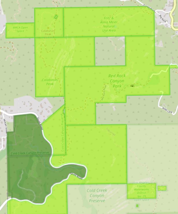
Because of these issues, we could not simply take the objects provided by PAD-US and call them “parks” for our analysis. Instead, we developed a series of geoprocessing steps to more consistently represent lands as parks. Our initial step was to explode the PAD-US data, converting all multi-part polygons into single parts. Using the individual park polygon pieces, we then rebuilt “clusters” based on adjacency, creating clusters of contiguous public lands that might be experienced as one “park.” When those clusters are over 100 acres, all parts are considered regional parks or open spaces for our analysis. This does not resolve all of the complexity because PAD-US is inconsistent in how records in the database are defined. Parks range from being a collection of hundreds of detailed parcels to massive multi-part polygons that cover hundreds of thousands of acres. In some states, U.S. Forest Service and BLM lands are highly detailed and broken down into small pieces. In others, they are one large polygon that is not broken apart unless it is multi-part. 

But overall, the results were meaningful and our approach worked in the vast majority of cases. It still created some enormous single clusters, such as all of the Eastern Sierra in California, from Mexico to Oregon. That’s much too large to experience as a single park. To rectify this, we split lands when they were: in the same cluster and had the same manager, name, and public access. In testing on some known areas, including several large national forests, this produced the best outputs and is our final methodology for analyzing regional parks and open spaces.

Even so, there are some edge cases in all our states:

• In some places, public lands data is messy and poorly attributed, so we still have “parks” that span large areas and multiple polygons. Although this results in discontiguous parks and visitorsheds, we are still able to count these in our analysis of regional park access, since they do provide public lands access, but we treat them as exceptions in our web application when a user requests a single visitorshed report for such lands, since the result would be highly scattered and difficult to compute dynamically.
• Areas that locals might perceive as one large park could be counted as multiple regional parks if the polygons were not contiguous. These large park could get split into both neighborhood parks (small polygons) and regional parks (large polygons) if they were discontiguous, and depending on their polygon sizes
• Note also that we didn’t define a minimum size for a park in this analysis. PAD-US includes slivers (tiny edges) but also legitimate pocket parks. These slivers tend to occur along state lines where geoprocessing can produce noise where layers do not align precisely along borders. Further complicating the issue of trying to define a minimum size is that fact that some regions of PAD-US include lands such as right-of-ways, landscaped medians, vacant/undeveloped city lots, utility corridors, and other “public” land that is classified as open but may not be a “park”.

A few other notes on park definitions:

• We treat all golf courses as restricted access, regardless of their classification in PADUS.
• PADUS contains some lands that are not fee-title parks. These are excluded from our analysis.
• Lands in PADUS can overlap. This can lead to minor overcounts in the number of parks people can access in a specific location, though in our review did not impact the most important locations (no park access) and did not materially impact whether areas were “low” or “high” relative to other locations.

Defining entry points

After using the methods described above to define regional parks and open spaces, we then moved to calculating "visitorsheds" of those parks. To do this, one must first determine how the public is able to physically enter public lands. We make an important distinction between neighborhood and regional parks. Neighborhood parks are considered to have predominantly permeable borders and thus we do not assign specific entry points. Regional parks more commonly have points of entry (parking lots, trailheads, etc) that can be used for routing estimates.

For example, Pinnacles National Park has very limited points of entry:

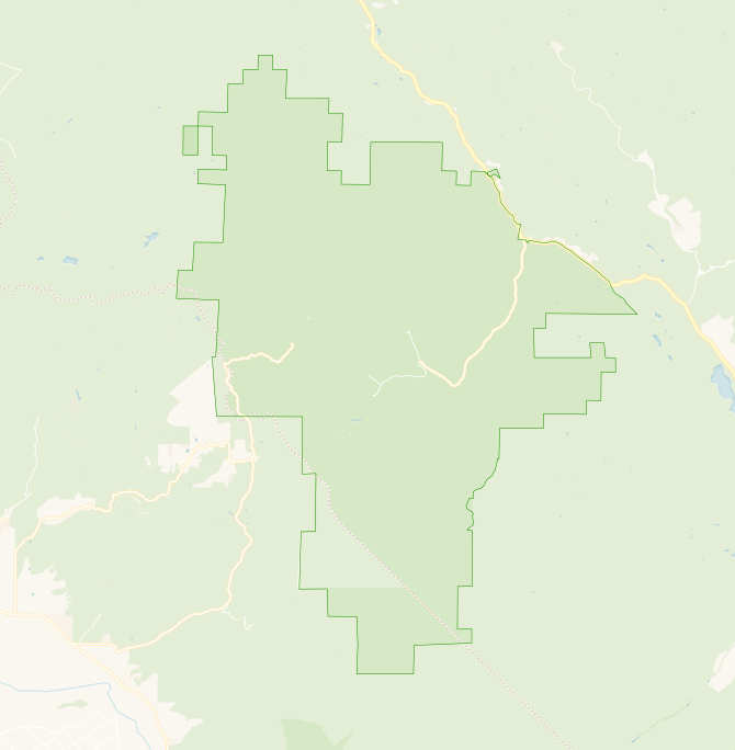
Unfortunately, there is no database of every trailhead, parking lot, ticket kiosk, roadside pullout, or sidewalk entry for the thousands of parks in any one state, much less multiple states. Lacking such a data source, we had to derive one that was sufficiently accurate for our purposes, knowing that it would not be completely accurate for all purposes.

To do this, we used OpenStreetMap, a volunteer-created open source map of the world, to intersect drivable roads with our park boundaries and create potential entry points. We refined this method by excluding certain classes of roads, such as divided highways and freeways, which often pass through public lands without providing access, unless there is an off-ramp (which would appear under a different class of roads). In many cases, a drivable road comes close to but does not actually intersect the edge of a park, but it still provides access via a connecting walkable pathway. To account for this, we also intersected non-drivable roads with parks, but only retained the entry points if they were within 1,000 feet of a drivable road. As in other cases, we still have seen edge cases where a road skirts or surrounds a park but does not intersect it in the data. In that case, we can't produce an entry point, and therefore can't produce a driveshed, and therefore don't count this park in our access metrics, though someone might still be able to walk into it from the surrounding road.

We knew that this dataset would be only an approximation of access, and we would never recommend using it to give anyone directions to a park. But in our testing and review, the approach produces results sufficient for local, regional, and statewide analysis when taking into account other mitigating factors we implemented when combining isochrones (areas within a defined driving distance of a single point) into drivesheds and then distributing demographic data based on where people live. Those items are explained in more detail in the following sections.

Defining Walking Visitorsheds

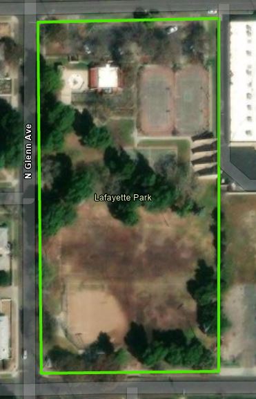
For Neighborhood Parks, we used a simple half-mile Euclidean buffer distance to define the walkshed for each park. By using Euclidean buffers we are able to assume that neighborhood parks are not entry point specific and instead buffer the full boundary of a park.

Also, we have found that network analysis for such small areas is of limited value. Network data for driving is much better than for walking. Accurate walkshed routing would require extensive improvements to data about sidewalks, crosswalks, and trails. In testing, we found hyperlocal network distance across both urban and rural landscapes often produces as many errors as it solves.

There is precedent for the Euclidean buffer method: It is the one used by the California Department of Parks and Recreation at parksforcalifornia.org. We took the proven approach here of a simple half-mile buffer from the park edge.

Defining Driving Visitorsheds

As described above, access to regional parks is most accurately represented by entry points. Entry points are also necessary to generate a network analysis that estimates the way people get to a park when using the road network. Network analysis is done using a technique of creating isochrones (areas within a defined network distance of a single point). We did this using an open source routing engine called Valhalla.

Using the entry points for each park (as described above), we were able to calculate the isochrones for each point where one could potentially enter a regional park. Each individual entry point isochrone could then be merged with other isochrones for that park or open space, and with the parent park, to produce a driving visitorhed.

To determine the distance people are willing to travel to visit a park we located a national survey about travel patterns. According to the National Household Travel Survey, the average recreational or social trip by car is 13 miles in urban areas and 23 miles in rural areas. 

Because many of the states in this project have distinct urban and rural areas, we felt it was important to distinguish which parks were urban and which were rural. The following methods were used:

• Each park entry point was used to create 13-mile isochrone and then merged to a respective park visitorshed.
• The 13-mile visitorsheds were evaluated to determine what percentage of the area was classified as urban or rural, according to the latest decennial Census block data (this was 2010 at the time of our analysis in 2022, since the 2020 version of this data had not been released yet). If a visitorshed was 50% or more urban, the park was considered urban and assigned a 13-mile visitorshed. 
• If the 13 mile visitorshed was less than 50% urban, a second test was run. The second test produced a 23-mile visitorshed and again looked at the percent urban versus rural. Those that were at least 50% urban also had their associated parks marked urban and assigned 13-mile visitorsheds. 
• All remaining parks were defined as rural and assigned 23-mile visitorsheds.

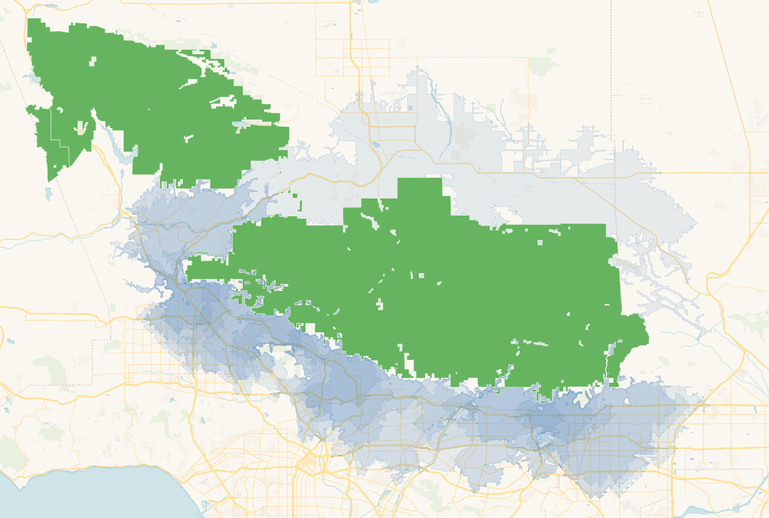
Once each park has been defined as urban or rural, the visitorsheds for associated groups of parks are merged to a single larger polygon that represents the visitorshed of one regional park or open space. That visitorshed is our estimated extent that  people would travel for an average recreational trip.

Every park visitorshed is the combination of many single point isochrones, and offers the additional benefit of diluting many potential issues with inaccurate entry points. In areas we surveyed that had some inaccurate entry points, we noticed that we also had nearby accurate points that covered the same area. When the isochrones were combined, the additional area covered by inaccurate points was negligible.

A note about transit

An obvious question for this project is why we are looking at walking distance for neighborhood parks and driving distance for regional parks, but not transit access for either one. There are a few reasons for this: First, the same National Household Travel Survey we used to understand typical driving distances also tells us that the typical recreational transit trip is 11 minutes, with no transfers. In the vast majority of locations, the number of regional parks and open spaces accessible that way is vanishingly small. Second, data availability for transit providers, while much better than in the past, remains challenging to assemble across entire states. Third, we do include demographic information about limited car access in our analysis, so in areas with limited car access, park advocates and decision makers can use that information to argue for improved transit services to parks and open spaces. And certainly, this project could be enhanced in the future by adding transit analysis to the work, though that is likely to be useful only in metro areas with already robust transit systems.

Understanding where people live

Based on all of the above, we knew not just where the regional parks and open spaces are, but also the areas from which they would most likely draw their regular visitors. But we didn’t yet know who lived in those areas — was this a dense urban neighborhood or a sparsely populated hinterland?

Typically, we use data from the American Community Survey (ACS) for this. The ACS provides an incredibly rich array of data about people in every part of the United States, usually at the Census Block Group level (and above). Each of those shapes have somewhere between 600 and 3,000 people in them. In urban areas, they are small but in rural areas they can be quite large.

Visitorsheds often cover large areas and have complex edges created by the road network analysis. To improve demographic reporting, we wanted to optimize our spatial analysis to more accurately account for where people do (and do not) live.

Several years ago, Meta (formerly Facebook) worked with academic and government patterns to develop the High-resolution Human Settlements Layer as a contribution to global humanitarian mapping and emergency response. The dataset uses high resolution satellite imagery combined with complex statistical analysis to estimate the population within each 30 meter grid cell across the Earth’s surface. The data is remarkably fine in detail, showing not only unpopulated forests and deserts but also allowing population estimates to account for the fact that that people don’t live on roads, at factories, or in malls or cemeteries, all areas where traditional census polygon boundaries would say that populations might be found, within some larger geometry.

Using these "People Points" allows us to estimate with much greater precision the populations and levels of park access for each 30m grid point across our pilot states.

This high-resolution data also helped us mitigate potential issues with inaccuracies in our entry point data (described above). In some areas where we estimated access would exist where it does not (for example, a road crossing a park boundary where you are not allowed to park or enter), we noticed the population was sparse or entirely absent in many of these same areas. So in that case, we didn’t actually overestimate access in those locations, because we only estimate access in places where people actually live.

The high-resolution data does have limitations, but the limitations did not outweigh the added value of more precise locations of population. Limitations include:

• Currently, the Human Settlements Layer people-points location data is from 2016. While this does mark a point in time for how the population is geographically distributed, we were able to use updated American Community Survey (ACS) 2019 demographics data allocated to the points. These methods are discussed in more detail in the next section.
• Limited demographic data is available from the Meta population data. Again, we are able to apply methods to improve this, as discussed below.
• Population totals for states tend to be shy of the official Census estimates, though most are within 5% of the population reported by the Census Bureau in 2016.

Assigning demographics

The Human Settlements Layer is highly detailed in its resolution but has two main limitations we aimed to improve. First we wanted more recent data, accomplished by factoring ACS 2019 population attributes to the 2016 distribution. Second, we wanted to include multiple topics such as race/ethnicity, educational attainment, income, and vehicle accessibility. Again, these data variables were possible to include by distributing 2019 data to the 2016 locations.

Recent population data was downloaded from the American Community Survey 2015-2019 block group data via the Census API. (While 2016-2020 data had been released, we were hesitant to accept the potential inaccuracies within the data due to COVID.) Once obtained, we were able to distribute population counts within block groups as follows:

For each population point, mark the block group it falls within

• Add the population points up, by block group - determining the number of people in the block group according to the population point data.
• For each population point, determine the percentage of the block group it represents
• Attached the ACS 2019 block group population data to each population point
• Derive the updated population for the point, by multiplying the percentage of the block group population from 2016 data, the ACS 2019 population. 

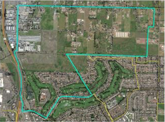
In the image below, the blue outline represents a Census block group, the smallest shape available for many Census metrics.  We know that  the polygon has 894 people inside it. With this image, we also see that it is visually obvious that the population is not evenly distributed. There are concentrations in the south and others sprinkled in the northern half. In urban areas the population concentrations are somewhat regular, though commercial areas can be skewed.

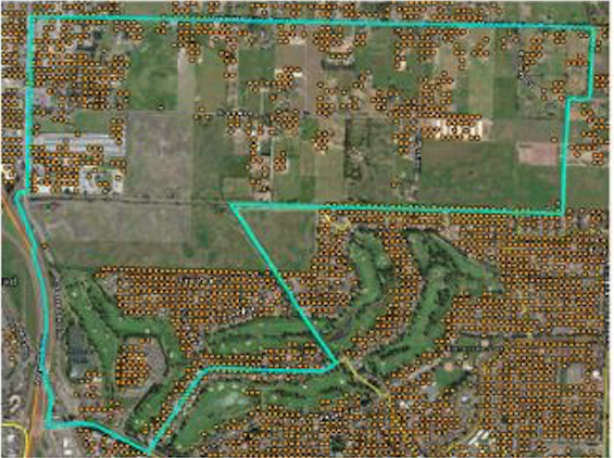
In the second image below, the Human Settlements Layer is more spatially detailed, showing the distribution of population on a 30 x 30 meter grid. In the same block group polygon, you can see the points are located where people live. In rural and suburban areas this can help highlight population concentrations and non-populated areas. Each point is attributed with the number of people at the location.

The second issue was the need to provide a wide range of attributes such as race/ethnicity, education, vehicle access, or any other number of things we can derive from the American Community Survey. This was possible by crosswalking the two datasets. Similar to the methods used to provide more current population totals, we were able to aggregate the population total from the Human Settlements Layer within a Census block group, and compute the relative number of other demographics. This method does have limitations. For example, if the 600 to 3,000 people within a block Group are themselves unevenly distributed among populated points, we won’t capture that in our analysis. This could occur if one side of a Block Group is dominated by one racial or ethnic group while the other is dominated by another. This means one should not use the data for neighborhood level outreach, but at that point talking to people on the ground is always better than using data. For initial planning and analysis, our data is the most detailed we have seen on such a wide spatial scale.

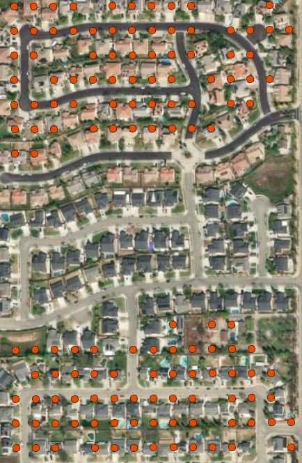
The other limitation is that we are distributing population to areas as mapped in the Human Settlement Layer, which could be missing areas with very recent construction. Because we are using the most recent ACS data, overall population estimates are the best available but in locations with rapid development or decline, spatial distribution of those populations might vary slightly at a local level. The example below highlights an area where housing has been built between 2017 and 2019, and is therefore not reflected in the points from 2016.

Estimating Park Access

Our final and perhaps most important step is to take our Park Visitorsheds, both Regional drivesheds and Neighborhood walksheds, and overlap them with our People Points. For every point, we calculated each of the following:

• How many Open Access Regional Parks or Open Spaces are accessible from this point
• How many Open Access Neighborhood Parks are accessible from this point
• How many Restricted/Closed Regional Parks or Open Spaces are accessible from this point
• How many Restricted/Closed Neighborhood Parks are accessible from this point

These numbers in turn support our overall policy recommendations of where investing in programs, opening restricted lands, or acquiring new lands would improve access for people who currently lack it.

Because our visitorsheds have noise at the edges of the road network, we use the data above only as an overall indicator of relative access, rather than a precise indicator of exactly how many parks one can reach from one 30 meter square vs the one next door.

Note that our metrics do not currently include a measure of what is often called park pressure, which attempts to measure the park "supply" compared to the number of people living nearby. This is often expressed as park acres per thousand people, and in California, the state set a threshold of at least 3 acres per thousand. We hope to add this measure to our data in the near future.

Glossary

Access to Car

Number of households responding they had no access to any vehicle. Census Source: ACS 2015-2019, data table B25044. Percentages are calculated using the Census-provide denominator appropriate to each measure.

Access to Internet

Household has a computer with dial-up or broadband internet. Census Source: ACS 2015-2019, data table B28003. Percentages are calculated using the Census-provide denominator appropriate to each measure.

Age, 18 to 64

Male and female population ages 18 to 64. Census Source: ACS 2015-2019, data table B01001. Percentages are calculated using the Census-provide denominator appropriate to each measure.

Age, 5 to 17

Male and female population ages 5 to 17. Census Source: ACS 2015-2019, data table B01001. Percentages are calculated using the Census-provide denominator appropriate to each measure.

Age, Senior (65+)

Male and female population ages 65 and over. Census Source: ACS 2015-2019, data table B01001. Percentages are calculated using the Census-provide denominator appropriate to each measure.

Age, Under 5

Male and female population under age 5. Census Source: ACS 2015-2019, data table B01001. Percentages are calculated using the Census-provide denominator appropriate to each measure.

Disability

Male and female population 20 to 64 with a disability (hearing, vision, cognitive, ambulatory, self-care, independent living). Census Source: ACS 2015-2019, data table B23024. Percentages are calculated using the Census-provide denominator appropriate to each measure.

Education, Bachelor's degree or higher

Male and female population 25 and older, have earned a bachelor's degree. Census Source: ACS 2015-2019, data table B15002. Percentages are calculated using the Census-provide denominator appropriate to each measure.

Education, High school grad or equivalent

Male and female population 25 and older, have earned a High School degree (including equivalent such as GED). Census Source: ACS 2015-2019, data table B15002. Percentages are calculated using the Census-provide denominator appropriate to each measure.

Education, Less than high school graduate

Male and female population 25 and older, education earned is less than a high school degree (or equivalent). Census Source: ACS 2015-2019, data table B15002. Percentages are calculated using the Census-provide denominator appropriate to each measure.

Education, Some college or associate's degree

Male and female population 25 and older, has earn college credits and/or an associate's degree. Census Source: ACS 2015-2019, data table B15002. Percentages are calculated using the Census-provide denominator appropriate to each measure.

Limited English Speaking Household

Household members have a limited ability to speak English. Census Source: ACS 2015-2019, data table C16002. Percentages are calculated using the Census-provide denominator appropriate to each measure.

Low Income

Median household income is below 80% of the state median household income. This is the same as the definition of Disadvantaged Communities (DAC) under California's landmark Assembly Bill 31 (2008), which set some of the nation's first measurable targets for equitable distribution of park funds. Census Source: ACS 2015-2019, data table B19001. Percentages are calculated using the Census-provide denominator appropriate to each measure.

Neighborhood Park

For this analysis, a neighborhood park is defined as any public land that is less than 100 acres that is also not contiguous with other public lands to create a cluster that would be larger than 100 acres. In most cases, these are familiar parks in the urban fabric: Small neighborhood parks surrounded by other kinds of development, and providing various levels of recreational facilities from simply an open field to playing fields and other infrastructure. Note that because we are using a size threshold, some small but remote public lands may be classified as Neighborhood Parks though very few people live nearby. 

Neighborhood Park Access

This measure represents the relative number of neighborhood parks within a half-mile of each point in our population data. We bucket each point into a quantile based on statewide data to compare areas with relatively high or low access. Read more in our About page on how we define parks, population data, and half-mile areas.

Race, American Indian and Alaska Native Alone

Population that is American Indian and Alaska Native Alone, not Hispanic or Latino. Census Source: ACS 2015-2019, data table B03002. Percentages are calculated using the Census-provide denominator appropriate to each measure.

Race, Asian Alone

Population that is Asian, Native Hawaiian and Other Pacific Islander alone, not Hispanic or Latino. Census Source: ACS 2015-2019, data table B03002. Percentages are calculated using the Census-provide denominator appropriate to each measure.

Race, Black Alone

Population that is Black or African American alone, not Hispanic or Latino. Census Source: ACS 2015-2019, data table B03002. Percentages are calculated using the Census-provide denominator appropriate to each measure.

Race, Hispanic/Latino

Population that is Hispanic or Latino. Census Source: ACS 2015-2019, data table B03002. Percentages are calculated using the Census-provide denominator appropriate to each measure.

Race, Native Hawaiian and Pacific Islander Alone

Population that is Native Hawaiian and Pacific Islander alone, not Hispanic or Latino. Census Source: ACS 2015-2019, data table B03002. Percentages are calculated using the Census-provide denominator appropriate to each measure.

Race, Other Race Alone

Population that is of other race alone, not Hispanic or Latino. Census Source: ACS 2015-2019, data table B03002. Percentages are calculated using the Census-provide denominator appropriate to each measure.

Race, Two or More

Population two or more races, not Hispanic or Latino. Census Source: ACS 2015-2019, data table B03002. Percentages are calculated using the Census-provide denominator appropriate to each measure.

Race, White Alone

Population that is White alone, not Hispanic or Latino. Census Source: ACS 2015-2019, data table B03002. Percentages are calculated using the Census-provide denominator appropriate to each measure.

Regional Park or Open Space

Regional Parks and Open Spaces are defined as either individual pieces of public lands that are greater than 100 acres or smaller areas that are clustered with adjacent lands that together form a contiguous public land area greater than 100 acres. See About for more important about methods and reasoning in this definition.

Regional Park or Open Space Access

This measure represents the relative number of regional parks and open spaces within the visitorshed of each point in our population data. We bucket each point into a quantile based on statewide data to compare areas with relatively high or low access. Read more in our About page on how we define parks, visitorsheds, population data, and half-mile areas around neighborhood parks.

Very Low Income

Median household income is below 60% of the state median household income. This is the same as the definition of Severely Disadvantaged Communities (SDAC) under California's landmark Assembly Bill 31 (2008), which set some of the nation's first measurable targets for equitable distribution of park funds. Census Source: ACS 2015-2019, data table B19001. Percentages are calculated using the Census-provide denominator appropriate to each measure.